Simulation of the Instability of Gas Layer Flow Inside Fluid Volume 1 - Issue 5

Іvan V Kazachkov*

• Department of Information Technologies and Data Analysis, Ukraine

Received:February 19, 2019;   Published:February 28, 2019

*Corresponding author:Іvan V Kazachkov, Dept of Information Technologies and Data Analysis, Ukraine

DOI: 10.32474/ARME.2019.01.000123

Abstract PDF

---

Abstract

The stability of a thin gas layer flow between two fluid layers moving in the same or opposite direction is modeled and simulated numerically. A linear stability is considered for the system using the non-stationary equation array, which consists of the two onedimensional non-stationary equations of a seventh and fourth order. The results of the numerical study showed that the thin gas layer between two liquid layers is unstable to a number of different perturbations of the flow parameters.

Keywords:Flow, Gas Layer, Liquid, Interface, Linear Stability, Three Layers, Instability, Interface

Introduction to the Problem

Gas or vapor layer flow may occur in a number of different physical facilities and devices [1-3], e.g. in a pool with volatile coolant [4,5]. Also, as a stage of drop disintegration through the phase of a film flow [6], etc. In fact, the first two phenomena may occur together in real cases [4,5]. Such liquid - gas (vapor) interfaces are prone to different types of instability. The jet’s stability increases in infinite medium by increasing viscosities of jet and medium [7-9]. Instability of thin gas layer between two fluid layers was not reported in the literature yet.

Problem Formulation

The aim of paper is studying the phenomenon through the mathematical modeling and computer simulation. Linear equations for the spatial-temporal dynamics of the gas-liquid interfaces are derived and the boundary conditions are stated. The equation array is solved numerically and analytically (for same limit cases), and several sets of the base states are found, and their linear stability properties are examined.

Mathematical Model of The System

2-D three-layer flow is considered for the following physical situation. In equilibrium state supposed to be three layers moving with constant velocities in the same or different directions. The lowest layer is considered being in the rest or the coordinate system is touched with it moving with the same velocity. So that gas layer is moving with respect to lower layer with velocity U₁. And the upper liquid layer moves with velocity U2 against gas layer or in the same direction (U₂ < 0). It is assumed that inertia forces are big enough to neglect gravitational forces. And y=0, y=a are the unperturbed interfaces at the beginning. Gas flow supposed incompressible. The scheme of a three-layer flow: y=0, y=a – free surfaces of a gas layer; y=-b₁, y=b₂ – free surface of the lower and top liquid layers, U₁, U₂ – flow velocities. The governing equations are the continuity and the momentum Navier-Stokes equations, which can be represented in the following linearized form:

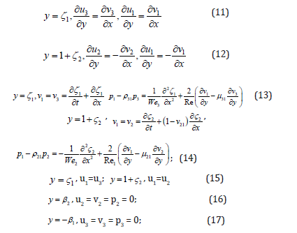
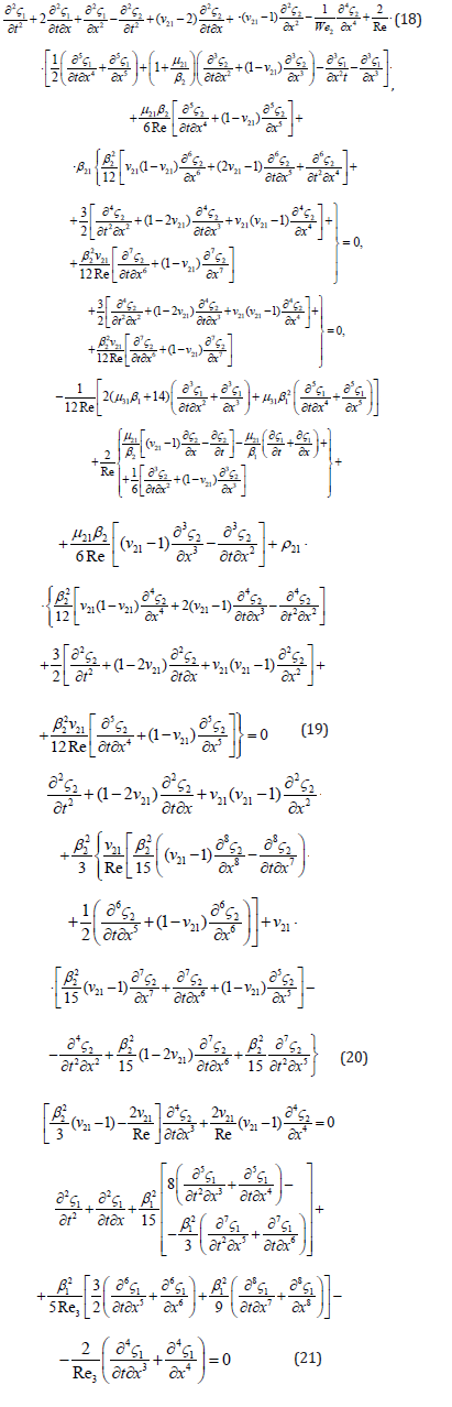
Where V = {U, V}is the fluid velocity field, p is the pressure, t is time, ∇ ≡ (∂_x,∂_y) , ρ - density, μ - dynamic viscosity and indexes, j = 1, 2, 3 are used for gas (vapor), top liquid and bottom liquid, respectively. Boundary conditions are following: tangential stresses supposed to be negligible at the gas – liquid interfaces, therefore

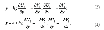
where h_j(x,t) are small-amplitude perturbations of the interfaces of the gas flow layer. The balances of the normal stresses at the interfaces and the augmented kinematics condition are:

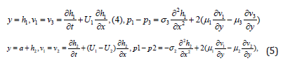
where σ₂ ,σ₃ , are the surface tension coefficients for the low and top liquid layers with a gas layer, respectively. In (4), (5) the capillary forces are taken with the opposite signs because convex and concave for the top and lower surfaces result in capillary pressure in a gas layer different by sign. Slip is neglected at the interfaces:

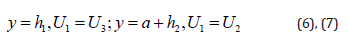
In unperturbed state the interfaces are the straightforward lines, there is a gas slip at the interfaces. But no-slip is considered by gas flow with the perturbed interfaces having uneven boundaries. The liquid layers supposed to be thick enough to suppress the perturbation inside them:

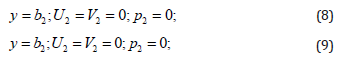
where b₁>>h₁, b₂>>h₂. The boundary conditions are linear in assumption that the long-wave small-amplitude perturbations of interfaces are considered. Boundary layer approximation may be applied for the thin gas layer. Then for gas flow p1=p1(x, t), and the momentum equation in y is omitted. Considering the instability of the interfaces one can integrate the equations (1) with boundary conditions (2)-(9) with respect to y and reduce the boundary problem (1)-(9) to the evolutionary equations for Then it is better to use a dimensionless form. The scale values are chosen as: a, U₁, a/U₁, p₁U²₁ 1 - for the length, velocity, time and pressure, respectively. It is considered that in the unperturbed state the layers move with constant velocities along x. Then dimensionless boundary problem (1)-(9) for perturbations is got in the following form:

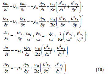
where the momentum equation for the gas flow is omitted because a boundary layer approach is adopted for it due to considered thin gas layer. Here Re =U₁ a /ν₁ - the Reynolds number for gas flow, ν - kinematic viscosity coefficient, ρ₁₂ = ρ₁/ ρ₂ ,ρ₁₃ = ρ₁/ ρ₃, ν₂₁=ν ₂ /ν₁ ,ν ₃₁ =ν ₃ /ν₁ , U₂₁ =U₂ /U₁ . Here U₂₁ characterizes the liquid to gas velocity ratio. Dimensionless boundary conditions (2)-(9) are

Mathematical Model of the System

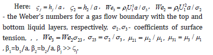
From (10)–(17), derivation of the evolutionary equations for oscillations of the boundaries of gas layer was done [9], with polynomial approximation of the transversal velocities in the layers. The following differential equations for the perturbations of boundaries of layers were obtained [9] as:

Problem Solution

Analysis of the system (18) - (21) allows stability study of the boundaries of gas flow. The partial differential equation array includes the derivatives from perturbations of the gas free surfaces by time t and coordinate x. It is seen that derivatives are of the higher orders up to the eighth order; therefore it is difficult for solving. Four equations totally, two functions sought, which is a consequence of the approximations applied for the profiles of transversal velocities and pressures of the liquid layers. As far as two last equations are autonomous, they can be solved independently, considering for example the simple harmonic waves in the form

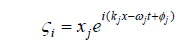
where j=1,2, i = −1 , x _j – constants, the initial amplitudes of the perturbations, k_j, w_j- the wave numbers and frequencies of the oscillations, φ_j – the initial phases of perturbations. Afterward, substituting the obtained solution into the other two equations of the system, we can get dispersion equations for computing the frequencies of perturbations w_j = w_j (k_j) depending on the wave numbers. The perturbations of the top and lower boundaries are interconnected and can differ only by the initial phases φ_j, k₁= k₂= k, w₁ = w₁ = w:

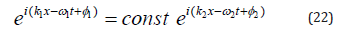
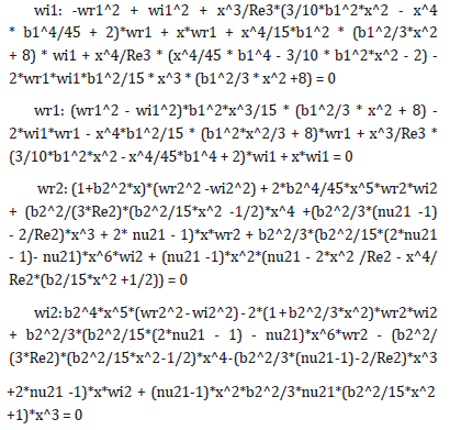
With account of the above, substituting (22) into (20), (21) after the contraction of the exponent and the amplitude xj (the equations are linear homogeneous in terms of the perturbations), we obtain:

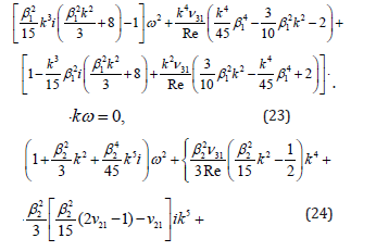
In the momentum equation for the second phase (upper liquid layer) the terms ln β₂ are kept, becauseβ₂ >> 1 can be by: ln β₂~ β₂ (e.g., β₂ =100 , ln β₂ ≈ 4,6 ; 2 β =10 , lnβ₂ ≈ 2,3 ; β₂ =1000 , lnβ₂ ≈ 6,9 ; 4 β₂ =10 , ln β₂ = 9, 2 obviously the terms with 2 lnβ ~ 1 , when β₂ ~ 10 , but ln β₂ ~ 10 for β₂ in a substantially wide range of β₂ . Thus, the terms with ln β₂ can be omitted when β₂ ~ 10 and β₂ ~ 1000 and higher, and around β₂ ~ 100 they can be substantial and depending of specific values because they are multiplayers with bigger ones than β₂ ). Further work must be done with computational experiment and analysis of the results obtained. The model thus derived may be useful in the investigations of some physical problems including stability of the vapor layer around the hot particle during its cooling in a volatile liquid, for revealing the peculiarities of the heat transfer critical heat flux. Computer Simulation of the Free Boundaries of Gas Layer Parameters of the available surface waves on the interface of gas layer with the liquid layers are computed from solution of the equation array (23), (24): k1= k2= k, w₁ = w₂ = w. Both, wave numbers and frequences of the oscillations are complex in a general case. For searching these values, the Flexed platform was used to prepare the computer program and provide the numerical simulation. The computer program was developed in the following form:

TITLE ‘3 fluids’ { the problem identification }

Select ngrid = 5 errlim = 0.001

variables

wr1 wi1 wr2 wi2

COORDINATES cartesian1 { coordinate system, 1D,2D,3D, etc }

definitions { system variables }

b1 = 1 b2 = 100 Re3 = 100 Re2= 12000 nu21 = 0.5

EQUATIONS { PDE’s, one for each variable }

{ one possibility }

BOUNDARIES { The domain definition }

REGION ‘domian’ { For each material region }

start (0) line to (10)

MONITORS { show progress }

PLOTS { save result displays }

elevation(wr1,wi1, wr2, wi2) from (0) to (1)

elevation(wr1,wi1, wr2, wi2) from (0.5) to (1.5)

elevation(wr1,wi1, wr2, wi2) from (1) to (2)

elevation(wr1,wi1, wr2, wi2) from (2) to (3)

elevation(wr1,wi1,wr2,wi2) from (0) to (10)

END

Here the values wr1, wi1, wr2, wi2 mean the real and imagine parts of the frequencies of perturbations. The argument x in the program means wave number k. The other parameters are: β₁ = 10, β₂ = 0.1 (thin gas layer), Re3 = 10⁶, Re2 = 5·10⁴ (Re2= Re· 21 v ), 21 v = 17.2 ·10^-6. The results of numerical simulation with the above computer program are presented below in Figure 1 as the graphs for real (wr1, wr2) and imagine (wi1, wi2) parts of the w₁, w₂ versus the wave number k (x in figures):

As far as equations (23), (24) are satisfied simulataneously, w₁=w₂ is available for the above stated parameters approximately by k = 0.5, which corresponds to the long-wave perturbations of the interface. The short waves do not satisfy the equation array and physically it is understandable because the short waves are fast decreasing with time. For the representing the corresponding surface waves , the following computer program was used:

TITLE ‘3 liquids’ { the problem identification }

Select ngrid = 5 errlim = 0.01

Variables e

COORDINATES cartesian1 { coordinate system, 1D,2D,3D, etc }

definitions { system variables }

wr1 = 2*10^-5 wi1 = 3*10^-5 k = 0.5

EQUATIONS { PDE’s, one for each variable }

e = exp(wi1*t)* (cos(k*x - wr1*t)

BOUNDARIES { The domain definition }

REGION ‘domian’ { For each material region }

start (0) line to (10)

TIME 0 TO 100 by 0.4 { if time dependent }

MONITORS { show progress }

PLOTS { save result displays }

for t = starttime by ( endtime - starttime) / 200 to endtime { snapshots }

elevation( e) from ( 0) to ( 20) as “e”

history (e) at (0)

END

The results of computation are presented in Figure 2, where from is seen that the wave is nearly of the same amplitude (just oscillation) by these parameters, only the thinner is gas layer, the higher are oscillations being still stable by these parameters. For the second case (β₁ = 1,β₂ = 0.1) the parameters are: wr1 = 2*10^-5, wi1 = 3*10^-5, k = 1.51, so that the perturbation of the interface is very slowly growing by time being nearly stationary (phase velocity of the surface wave is approximately 1.3*10^-5). The other results support the mentioned. Calculation for t = 7.5*10⁴ gave the same result as for t = 5*10⁴. Both correspond to complete disintegration of the gas layer. Both graphs (by time at x=0 and by x depending on time show the same results of the system’s instability).

Figure 2 Wave e^{i(k1x−ω1t+φ1)} against time by x = 0 and against x at the moment t = 5*10⁴ (β₁ = 1, β₂ = 0.1). Instability is developed up to destroying the system on the drops and fragments in the time about t=2 (about ten times growing of the oscillations by amplitude; the time is dimensionless; therefore it depends on parameters: width of the layer and velocity of the flow). Red colored are parameters ω in the table below, which correspond to the growing (unstable) perturbations, while the blue ones - to the stable oscillations.

Using the results obtained one can study the influence of the parameters on stability of the gas layer moving between the liquid layers. As shown above, mostly it is unstable. The results may be treated as instability of the vapor layer surrounding the hot liquid drop, which is cooled down in a volatile coolant, for example under severe accident at the nuclear power plant (Table 1).

Conclusion

As numerical simulation revealed, all values of the ω are complex. The imagine part of frequency ω means that by positive values of ω the perturbations are growing by time (instability) or fading (stability). By real frequency when imagine part is absent, the perturbations are just oscillating interfaces between the layers. Thus, we have got many parameters of the perturbations, which lead to the breaking the gas layer.

For example, by β₁=2, β₂=2 and v=10, the system is stable. Mainly stable regimes are observed by the next parameters:

β₁=2, β₂=0.5, v=100;

β₁=0.5, β₂=2, v=10;

β₁=1, β₂=0.5, v=10;

β₁=2, β₂=2, v=100;

β₁=2, β₂=2, v=1000;

β₁=0.5, β₂=0.5, v=10.

But in reality the system is unstable if there are just a few available unstable oscillations of the interface because many of them are present. Therefore, the conclusion is that gas layer moving between the liquid layers is unstable and the most unstable waves are of the length a few width of the gas layer.s

References

1. HS Park, IV Kazachkov, BR Sehgal, Y Maruyama, S Fujui (2001) Analysis of plunging jet penetration into liquid pool with various densities. Fourth International Conference on Multiphase Flow, New Orleans, Louisiana, USA.
2. KA Bin (1993) Gas entrainment by plunging liguid jets. Chem Eng Sci 48(21): 3585-3630.
3. H Chanson (1996) Air Bubble Entrainment in Free-Surface Turbulent Shear Flows. Academic Press, San Diego, CA.
4. HS Park, N Yamano, K Moriyama, Y Moruyama, Y Yang, et al. (1998) Study on Subcooled water injection into molten material. Heat Transfer 6(69): 1998.
5. SJ Board (1975) Detonation of Fuel Coolant Explosions. Nature 254(319): 1975.
6. BE Gelfand (1996) Droplet breakup phenomena in flows with velocity lag. Prog. Energy Combust Sci 22(3): 201-265.
7. S Tomotika (1935) On the instability of a cylindrical thread of viscous liquid surrounded by another viscous fluid. Proc Ray Soc (London), 150: (322).
8. BJ Meister, GF Shecle (1967) Generalized solution of the Tomotika stability analysis for a cylindrical jet. AICRE Journal 13(4): 682-688.
9. Ivan V Kazachkov (2018) The dynamics of thin gas layer moving between two fluids. USA: Cornell University. ArXiv: 1803.05175.